MapReduce

http://static.googleusercontent.com/media/research.google.com/en//archive/mapreduce-osdi04.pdf

Introduction

Use cases
- At Google: process large datasets to generate
  - Inverted indices
  - Graph structure of web page links in various forms
  - Summarize crawl statistics per host
  - Most frequent queries per day
- In general:
  - Large scale ML
  - Clustering problems (Google News)
  - Extracting data for Google Zeitgeist
  - Extract data from web pages (eg. location clues for localized search)
  - Large scale graph computations
- Others
  - Distributed grep: map performs local filtering, reduce is a no-op
  - Reverse web-link graph: map outputs (target, source) pairs for each link to target in a source page. Reduce concatenates to end with (target, list(source)) pairs.
  - Inverted index: Map produces (word, document ID) pairs, reduce concatenates & sorts to end with (word, list(doc ID)).
MR is an abstraction that attempts to hide the impl. details of parallelization, fault-tolerance, data distribution, and load balancing for batch computation
The design is optimizing for network bandwidth above all else
We realized that most of our computations involved applying a map operation to each logical “record” in our input in order to compute a set of intermediate key/value pairs, and then applying a reduce operation to all the values that shared the same key, in order to combine the derived data appropriately.
Re-execution is the primary mechanism for fault-tolerance
Intermediate output can be larger than memory

Pseudo-code for word-count MR functions:

map(String key, String value):
	# key: document name 
	# value: document contents for each word w in value:
	EmitIntermediate(w, "1")

reduce(String key, Iterator values):
	# key: a word
	# values: a list of counts
	int result = 0
	for each v in values:
      result += ParseInt(v)
      Emit(AsString(result))

Many implementations are possible based on the computing environment.
Google uses clusters of PCs connected by switched Ethernet.
- Dual-processor x86, Linux, 2-4GB RAM. (Cores?)
- Commodity networking, 100 megabit - 1 gigabit per machine.
- Clusters contain 100s-1000s of machines, so failures are common
- Storage is entirely on spinning disks via IDE (2004!)

Implementation

Execution

Execution Overview

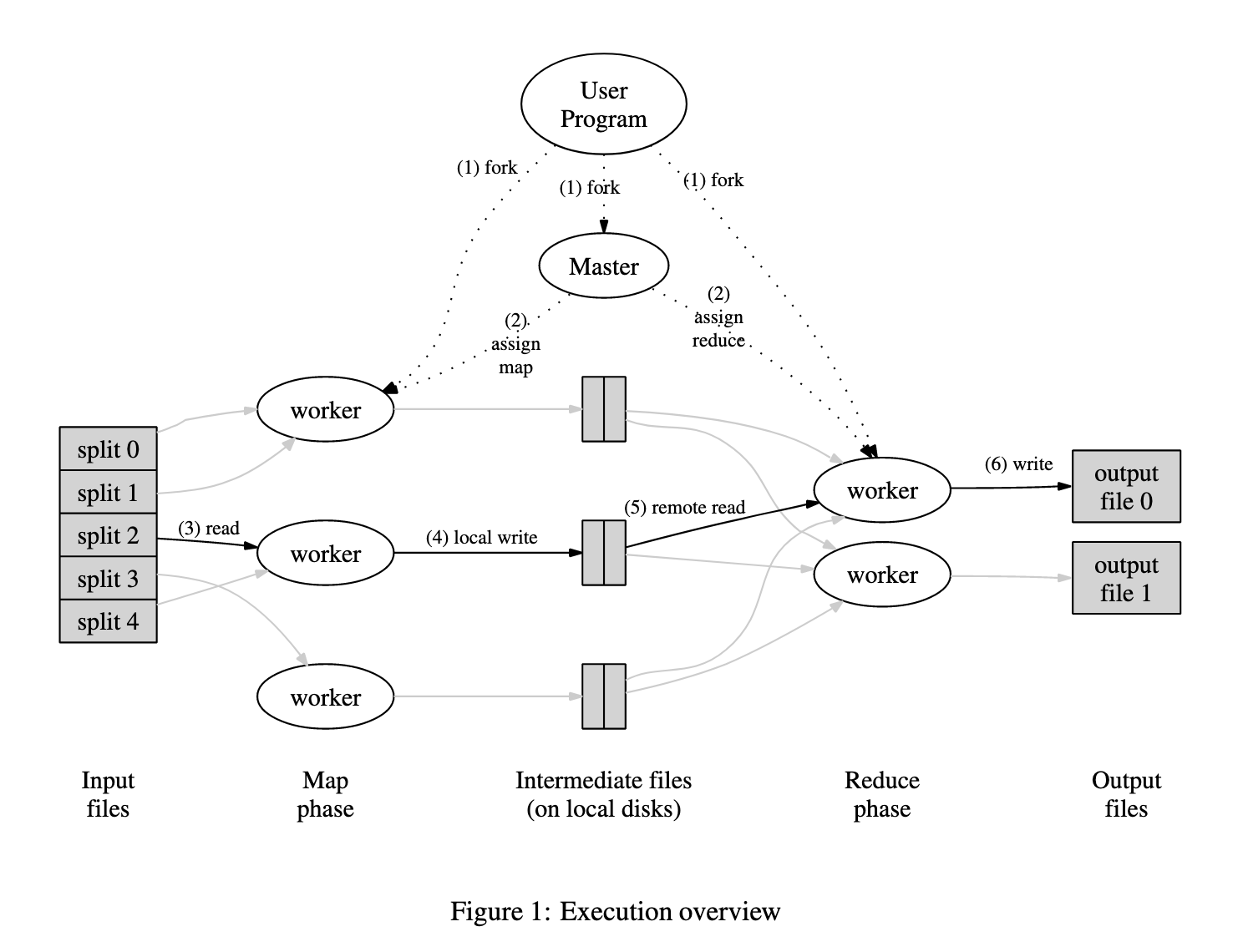
Partition input data into $M$ splits; this is the number of map operations
The number of reduces $R$ is manually set, but can’t be larger than the number of unique intermediate $K$s. A partitioning function translates from the keyspace to a given instance of the reduce fn.
$M$ and $R$ should ideally be much larger than the number of worker machines. The master makes $O(M + R)$ scheduling decisions and stores $O(M * R)$ state in msortemory, so there’s a tradeoff here to consider.
- $R$ is generally kept small because it controls the number of output files
- $M$ is typically set to the number of 64MB chunks you can divide your input into
- Google often uses $M = 200,000$ and $R = 5,000$ with 2000 workers
Each worker can perform different tasks; there aren’t technically disjoint sets of “map workers” and “reduce workers”.
Intermediate output is divided into $R$ sections; each reduce worker grabs its section from each map worker’s output, combines all these files, and sorts them (possibly not in-memory) by key.
The reduce worker then iterates over this sorted output and passes all values for each key to the reduce fn. Output is appended to a single output file for this worker.
Final output is $R$ files
The master receives locations of intermediate output as map tasks complete. This data is incrementally passed to reduce workers.
- This seems to imply that a reduce worker can start processing intermediate output (but not finish the entire reduce) before all maps are done.
- Not sure if the reduce worker can do anything except downloading intermediate output (+ possibly start sorting if using an incremental sort like merge sort) until all maps are done.
Stragglers can hurt overall performance - one worker that is struggling, for example
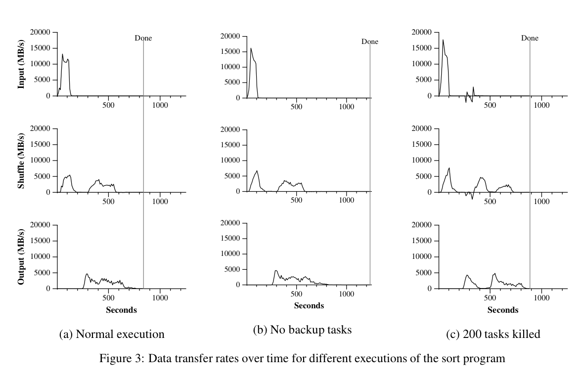
- When the entire job is close to completion, the master schedules backup executions of the remaining in-progress tasks, and output from either the backup or the original executions can be used.
- Backup-less execution has caused slowdowns on the order of 44% for some jobs.

Fault Tolerance

The master pings each worker; workers that don’t respond are marked failed
- All completed map tasks on the worker are marked “not started”
- All in-progress tasks on the worker are marked “not started”
If a map task is re-executed, all reduce workers need to be notified.
The master can checkpoint itself and be failed over manually, but Google uses the simple approach here and just fails the job if the master goes do.
When map and reduce are pure, MR will produce the same output as a sequential single-node implementation.
- This is possible by having map and reduce workers mark completion atomically, by using temporary files and renaming them at the end.

Locality

GFS splits up data into 64MB chunks and replicates them (rf=3), so the master tries to assign map tasks to workers in a way that maximizes reads off local disks.
If that isn’t possible, the next best thing is to read a chunk from a “closer” machine, which might mean a machine connected to the same switch.

Custom partitioning logic so all URLs from a given host go to the same reducer (and therefore the same output file), for example
Reducers sort by key before running the reduce operation, so they could also sort by (key, value) to provide ordering guarantees per-key.
A combiner function is a piece of code that perfoms early/partial processing during the map task.
- The same function can be (this is typical) passed as both the reduce and combiner functions.
- For the word count job, this converts thousands of (the, 1) entries in the intermediate output for a single map task to a single (the, 5000) entry, for example.

Performance

In this section we measure the performance of MapReduce on two computations running on a large cluster of machines. One computation searches through approximately one terabyte of data looking for a particular pattern. The other computation sorts approximately one terabyte of data.

These two programs are representative of a large subset of the real programs written by users of MapReduce one class of programs shufﬂes data from one representation to another, and another class extracts a small amount of interesting data from a large data set.

Test config
- 1800 machines, 2GHz Xeon, 4GB RAM (1-1.5GB used for other tasks on the same cluster), 2x160GB HD, gigabit ethernet
- Two-level tree-haped switched network, 200Gbps bandwidth at the root
- All machines in the same datacenter, <1ms latency
Grep
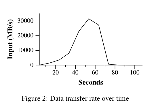
- Scan through $10^{10}$ 100-byte records; the pattern appears in ~92k records
- 150 seconds in total, including 1 minute in start-up overhead (!)
- Overhead includes: propagating the user code to all workers and GFS overhead for calculations around locality optimization
Sort
- The map function extracts a sort key and emits (sort key, record)
- The reduce function is a no-op
- The ordering guarantee (see
  Paper
  Refinements) gives us a sorted set of values per key.
  - Not sure I understand this (⌄⌄⌄⌄⌄); doesn’t the sort key implicitly define these split points? 🤔
    
    Our partitioning function for this benchmark has builtin knowledge of the distribution of keys. In a general sorting program, we would add a pre-pass MapReduce operation that would collect a sample of the keys and use the distribution of the sampled keys to compute splitpoints for the ﬁnal sorting pass.
  - In the image above:
    - The top row is the rate at which input is read
    - The middle row is the rate at which data is sent from the map tasks to the reduce tasks
    - The bottom row is the rate at which sorted data is written to the final output files
    - Reduce tasks receive data before all map tasks are done, but output doesn’t happen until all map tasks are done
    - Final output rate is relatively low because it (synchronously) writes to GFS at rf=2

Experience

MapReduce was used at the time of writing to build Google’s search index
Raw crawl data (20TB) is put into GFS and used as the initial input
Indexing is composed of 5-10 MR jobs in series

Conclusions

We have learned several things from this work.

First, restricting the programming model makes it easy to parallelize and distribute computations and to make such computations fault-tolerant.

Second, network bandwidth is a scarce resource. A number of optimizations in our system are therefore targeted at reducing the amount of data sent across the network: the locality optimization allows us to read data from local disks, and writing a single copy of the intermediate data to local disk saves network bandwidth.

Third, redundant execution can be used to reduce the impact of slow machines, and to handle machine failures and data loss.

Introduction

Implementation

Execution

Fault Tolerance

Locality

Refinements

Performance

Experience

Conclusions