Math

Derivatives

Instantaneous rate of change: how fast is something going right now, not an average measurement.
Slope == average rate of change. Assuming time on the X-axis and distance on the Y-axis, with a straight line representing distance covered:
```
$\text{Rate of change in distance} = \frac{\Delta y}{\Delta x} = \text{slope}$
```
This works fine when you’re dealing with a straight line (avg), but how do you apply this when you have a constant stream of instantaneous measurements and the graph is a curve, not a straight line? Essentially, take infinitesmally small measurements:
```
$\lim_{\Delta x\to0}\frac{\Delta y}{\Delta x}$
```
Also known as the derivative, again, conceptualized as an infinitely small change in y over an infinitely small change in x:
```
$\frac{dy}{dx}$
```
A straight line has a constant rate of change; the slope doesn’t change. A curve has a rate of change that’s continously changing; the rate of change at a given point is the slope of a tangent to the line drawn at that point.
Notation variants (all these are equivalent):
```
$\frac{dy}{dx} = f'(x_1) = \dot{y} = y'$
```
distance over time → speed over time (first derivative) → acceleration over time (second derivative)
Derivative of a function; given an $x$, choose a higher value $x+h$. The slope of the tangent at $x$ is:
```
$f'(x) = \lim_{h\to0}\frac{f(x+h) + f(x)}{h}$
```

Ref

https://www.khanacademy.org/math/differential-calculus/dc-diff-intro

Monte Carlo Method

https://en.wikipedia.org/wiki/Monte_Carlo_method

Monte Carlo methods, or Monte Carlo experiments, are a broad class of computational algorithms that rely on repeated random sampling to obtain numerical results. The underlying concept is to use randomness to solve problems that might be deterministic in principle

Monte Carlo methods vary, but tend to follow a particular pattern:

Define a domain of possible inputs

Generate inputs randomly from a probability distribution over the domain

Perform a deterministic computation on the inputs

Aggregate the results

For example, consider a quadrant (circular sector) inscribed in a unit square. Given that the ratio of their areas is π/4, the value of π can be approximated using a Monte Carlo method:

Draw a square, then inscribe a quadrant within it

Uniformly scatter a given number of points over the square

Count the number of points inside the quadrant, i.e. having a distance from the origin of less than 1

The ratio of the inside-count and the total-sample-count is an estimate of the ratio of the two areas, π/4.

Multiply the result by 4 to estimate π.

Phi Coefficient

From Wikipedia:

The phi coefficient (or mean square contingency coefficient and denoted by φ or rφ) is a measure of association for two binary variables

Given two binary variables, their interplay can be tabulated (for example, the top-left cell is some quantity when {{< m x >}} and {{< m “y” >}} are both true):

	x=1.	x=0	total
y=1	$n_{11}$	$n_{10}$	$n_{1\bullet}$
y=0	$n_{01}$	$n_{00}$	$n_{0\bullet}$
total	$n_{\bullet1}$	$n_{\bullet0}$	$n$

Now you calculate the phi coefficient like so:

$\phi = \frac{n_{11}n_{00}-n_{10}n_{01}}{\sqrt{n_{1\bullet}n_{0\bullet}n_{\bullet0}n_{\bullet1}}}$

or:

$\phi = \frac{nn_{11}-n_{1\bullet}n_{\bullet1}}{\sqrt{n_{1\bullet}n_{\bullet1}(n-n_{1\bullet})(n-n_{\bullet1})}}$

The result is a number in $[-1, 1]$ that indicates the degree to which $x$ and $y$ are associated/correlated. $1$ indicates that the variables are identical, and $0$ indicates that they’re effectively independent.

An example:

$x$: Event definition A
$y$: Event definition B
$n_{11}$: Number of events matching both event definitions

Power Law

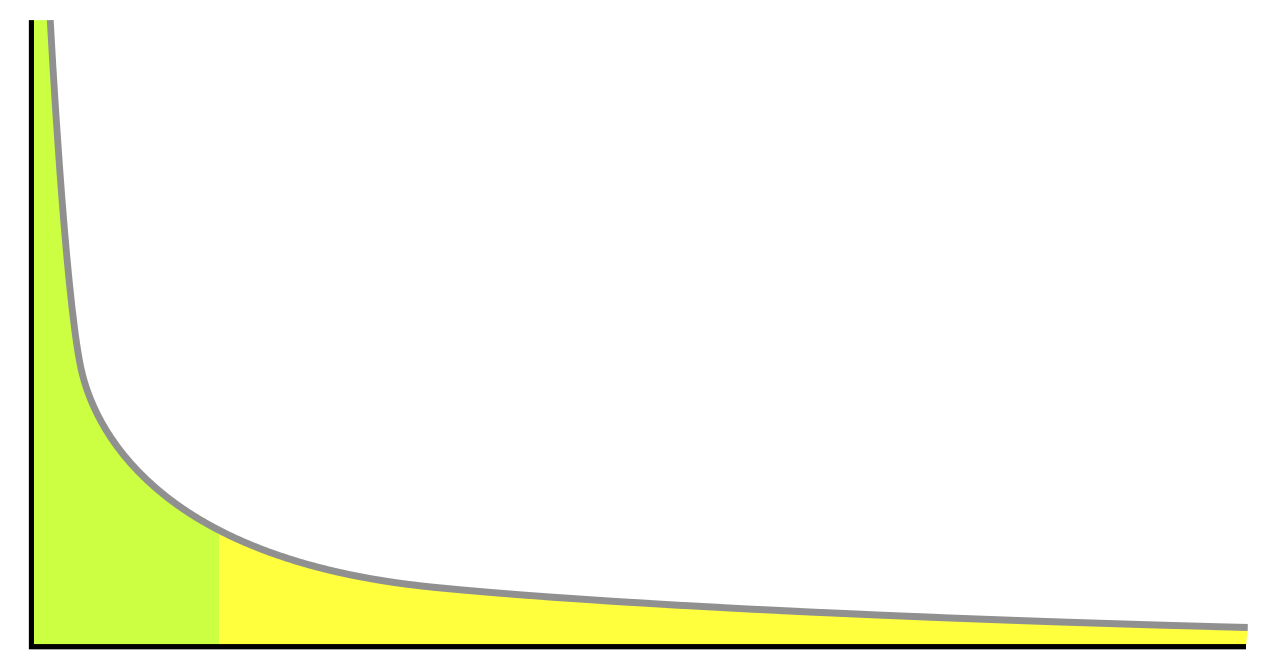
In statistics, a power law is a functional relationship between two quantities, where a relative change in one quantity results in a proportional relative change in the other quantity, independent of the initial size of those quantities: one quantity varies as a power of another.

A power law distribution has the form Y = k Xα, where:

$X$ and $Y$ are variables of interest,

$α$ is the law’s exponent,

$k$ is a constant.

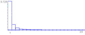
The power law can be used to describe a phenomenon where a small number of items is clustered at the top of a distribution (or at the bottom), taking up 95% of the resources. In other words, it implies a small amount of occurrences is common, while larger occurrences are rare. For example, where the distribution of income is concerned, there are very few billionaires; the bulk of the population holds very modest nest eggs.

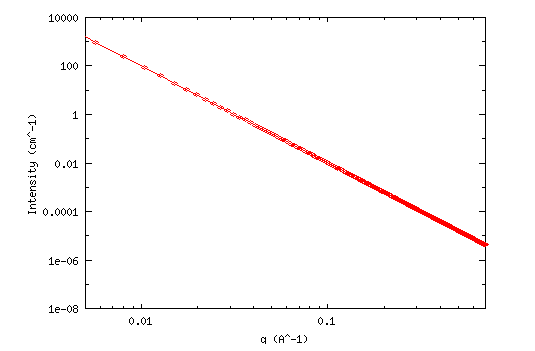
This is neat:

If you plot two quantities against each other with logarithmic axes and they show a linear relationship, this indicates that the two quantities have a power law distribution.

References

Slope

The slope or gradient of a line is a number that describes both the direction and the steepness of the line.
An upward-facing line has a positive slope, a downward-facing line has a negative slope.
The slope of a horizontal line = 0
The slope of a vertical line = undefined